IFRS 17 – the new revolutionary standard which aims to achieve comparability between insurers – may somewhat adversely impact that comparability by allowing considerable flexibility in estimating the discount rate curve used. The discount rate has significant implications on the financial statements of insurers. The complex structure of cash flows in certain contract groups, in combination with the average duration of contracts, may cause the present value to be highly sensitive to the discount rate used. In view of the typical high leverage level of insurers, it is clear that such measurement changes may trigger substantial variation in equity across the industry.
We believe that the standard should have created a certain hierarchy between the approaches it proposes, or a more comprehensive guidance of the manner of estimating the illiquidity premium and the required adjustments, as well as of the considerations to be taken into account when selecting and implementing the approaches IFRS 17 suggests for estimating the discount rate. The current situation begs the question – whether and how will the vacuum that has been created be filled?
Background
The highly complex insurance industry and the immense power wielded by the companies comprising it has made it difficult to form a global standard for reporting the financial position and results of operations of insurers. In 2004 – in an effort to reach a compromise in the lead up to the mandatory adoption of International Financial Reporting Standards (IFRS) by the European Union in 2005 – the IASB issued IFRS 4, which effectively enabled all insurers to continue using their original reporting formats (subject to certain adjustments and to the so-called “liability adequacy testing”, or LAT). Among other things, companies were allowed to apply conservative accounting policies. Accounting policies based on historical values when accounting for insurance contracts were also allowed.
After IFRS 4 came into effect – along with the mandatory application of IFRS in the European Union – a project was launched to develop a more comprehensive accounting standard for accounting for insurance contracts. One of the principal objectives of this process was to create of a unified accounting treatment for the entire insurance industry. However, the process appears to have been more complicated than expected: Almost 20 years later, this process gave rise to IFRS 17 (hereinafter – the “Standard”), that was already amended in 2020, even before its effective date in 2023 (after the said amendment and subject to the specific endorsement processes in the various jurisdictions, such as the EU).
Indeed, one wonders if this standard will lead to the desired result of accounting standardization. On the one hand, the standard will clearly reduce variance between financial statements of insurers. On the other hand, in addition to its inherent complexity, it appears that the standard allows a high level of flexibility, at least in certain aspects, which could make the analysis of the financial statements more difficult.
The aim of this article is to discuss one of the most material points of insurance companies’ financial reporting – the discount rate issue. Generally speaking, it should be noted that the generation of earnings from the following two fundamental components is an integral part of insurers’ activities:
- The first fundamental component is the underwriting or “insurance earnings”, which can be intuitively explained as the earnings generated from the fact that the expected present value of the claims is lower than the premium received from policyholders;
- The second fundamental component is investment earnings. These earnings, which sometimes constitute a substantial part of the insurers’ results, stem from the fact that sometimes there is a time difference between the cash inflows and outflows. The investment of premiums received from policyholders over the period until the payment of claims is a potential source for additional profits, or, in some cases, losses. In certain insurance segments, such as liability insurance, this timing difference may extend over years, enabling the insurer to generate substantial earnings from investment of premiums.
One of the most significant difficulties insurers face when reporting their financial results is how to separate between the said sources of earnings. From the perspective of financial statements’ users, such separation may help to separate recurring results from non-recurring ones – for example, higher than normal capital market earnings. This is further complicated when accounting for profit-participating insurance contracts. Another challenge stems, naturally, from the timing of the recognition and the period over which earnings are recognized in the statement of comprehensive income.
As part of the calculation of insurance reserves, future insurance claims (and expected proceeds and other cash flows) should be discounted. It is a rule of thumb that in insurance contract portfolios where premium is received in advance to the payment of expected claims, using a high discount rate will cause a decrease in insurance liabilities. In such case, new insurance contracts may also seem more profitable at inception. On the other hand, using a higher discount rate also inherently triggers more substantial expenses in the future, in respect of the passage of time (e.g., the higher the discount rate, the lower insurance liabilities are initially; however, they also increase at a higher rate because of the effect of time). Under a presentation method in which the said revision is separated from the other re-measurement effects and presented under finance expenses, it is obvious that this also reduces earnings from investment activities (the so-called spread between the implied discount rate and actual yield), which are composed of actual investment revenues net of the said finance expenses. Using a zero discount rate will cause a situation where the investment activity reflects all earnings from investments, without taking into account a “normative” deduction in respect of the interest component implicit in insurance contracts. The issue of the discount rate to be applied to insurance liabilities (or to insurance contracts as a whole) becomes even more pertinent when we also take into account the question of whether to use historical discount rates or current discount rates.
Obviously, using current discount rates may improve the relevance of financial statements, especially the statement of financial position, and especially in situations where the backing financial assets are measured at fair value (FVOCI or FVTPL) as well as other potential investments (such as investment property). In order to clarify this issue, let us take as an example an insurer issuing an insurance contract for which it charges a premium of EUR 926 and is required to pay the policyholder an expected value of total of EUR 1,200 after four years (an implicit yield of 9%). The insurer invests the entire premium amount in bonds with a four-year duration measured at fair value and generating a 9% yield. After one year, the bonds’ yield drops to 5%. In this situation, the insurer will recognize significant earnings from the appreciation of the bonds. Nevertheless, if the insurer continues to use the original discount rate for the insurance liability (say 9%), it will not recognize a loss from the appreciation of the liability, even though it is more difficult to achieve such a yield in the second year due to the decrease in market interest rates; this results in a mismatch and irrelevant equity.
In that context, it should be noted that IFRS 4 in its present form does not require the use of current discount rates or any discount rate at all, not even for the purpose of the liability adequacy test (LAT). It should be noted that the effect of the discount rate used on the insurance liabilities – and hence on the insurer’s equity – is very substantial. For certain liability types – such as life insurance, annuities or long-term care insurance – contracts may have average durations of 20, and sometimes even 40, years or more. The complex structure of cash flows in certain contract groups, in combination with the average duration of contracts, may cause the present value to be highly sensitive to the discount rate used. Thus, sometimes a one percent change in the discount rate may be sufficient to trigger a change of ten percent or more in certain insurance liabilities. In view of the typical high leverage level of insurers, it is clear that such measurement changes may trigger changes of tens of percent in equity and may, for instance, double the insurers’ equity or alternatively reduce it to zero.
The material effect of discount rates on financial statements, as well as the powerful interests at stake, were evident in the process of developing the US GAAP counterpart of IFRS 17. As part of this amendment (ASU-2018-12), which was also developed after discussions with numerous parties, the Financial Accounting Standards Board (FASB) opted to unify the discount rates used to measure insurance liabilities of long duration insurance contracts under US GAAP.
Under the ASU, an insurer will measure the liability for future policy benefits by using a discount rate that is based on the yield of an “upper-medium-grade” (low-credit-risk) fixed-income instrument (which would be the equivalent of an A-rated security). This model differs from the current guidance in US GAAP that uses a discount rate that is based on the insurer’s estimate of the anticipated investment yield on the underlying asset portfolio.
According to the ASU’s basis for conclusions, the main rationale behind this move was to increase comparability, operability, and to use objective market data. In this context it is interesting to note that the underlying yield curve was changed as part of the development of the ASU. In the original 2016 proposal the underlying yield curve was supposed to be “high quality” (equivalent to a AA-rated security). However, the yield curve was changed to upper-medium-grade in the final ASU, after receiving feedback from preparers of financial statements, as described in Section BC60 of the ASU. In many cases, this change will likely increase the insurance companies’ equity and will also cause new long duration business to appear more profitable.
Discount Rate: The Approach under IFRS 17
In this article we will not elaborate on the full accounting treatment set out in the Standard. Nevertheless, it should be emphasized that the main, albeit not the only, effect of the discount rates in the Standard is reflected in the measurement of insurance liabilities – specifically – the measurement of the discounted cash flow component underlying the insurance contract, plus the required risk adjustment in respect of non-financial risk – which amount to the so-called “fulfillment cash flows”.
IFRS 17 took one further step by determining that current market discount rates – rather than historical discount rates – shall be used to estimate insurance liabilities – which is similar to the conclusion reached by the FASB. Indeed, this may increase the relevancy of the balance sheet (see also Section BC192).
In principle, the Standard’s approach (which is similar to that of ASU-2018-12), especially with regard to liabilities that are not yield-dependent, is to decouple the measurement of insurance liabilities from the actual backing asset portfolio and the insurer’s past investment experience, as well as its own credit risk. Sections BC-200-201 of the Standard’s basis for conclusions state specifically that linking the backing assets to the liabilities (an asset-backed discount rate) is inappropriate, because there is no connection in the cash flows. Similar statements are made in Section BC61 of the explanatory notes to ASU-2018-12.
In our opinion, this stipulation of the Standard does, indeed, lead to a result that is relevant to users of the financial statements, since otherwise we would have ended up with a different estimate of the liabilities only due to a different composition of backing assets or a different investment experience. Furthermore, it appears that this principle is also in line with other accounting standards, such as IAS 19 (where the “high quality corporate bonds”, or HQCB, yield curve is used). As mentioned above, this principle is also broadly in line with the approach adopted by the FASB, as described above. However, and as described below, it appears that there are material differences in the level of flexibility allowed under each standard in terms of estimating the yield curve itself. By the way, it should also be noted that, with regard to yield-dependent or profit-participating liabilities – which this article will not expand on – there are stochastic approaches and approaches based on risk neutral modelling, whereby it is appropriate to use discount and expected yield rates which are risk-free in nature even when the backing portfolio includes investments which are not risk-free.
Indeed, despite the significant shift to using market data, it appears that the Standard still leaves extensive room for exercising judgement when deciding which approach to use to determine discount rate, and even what exactly this discount rate curve should represent. Specifically, with regard to liabilities that do not vary based on return on assets, the Standard mentions two approaches:
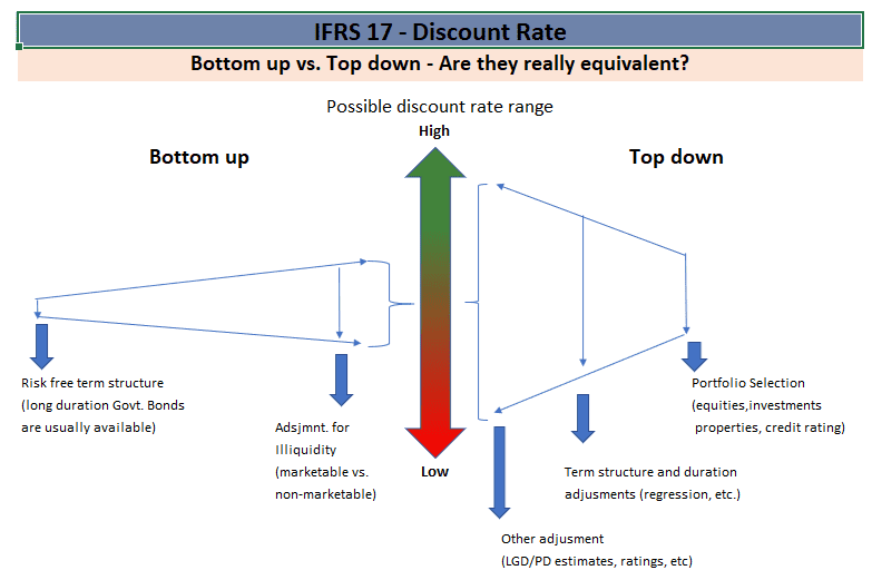
(a) The bottom-up approach – this approach, which is referred to in Section 80, uses a risk-free interest rate adjusted to reflect the illiquidity of insurance liabilities. Normally, a risk-free interest rate is based on observations taking into account factors such as swaps and yields on liquid government bonds. One should bear in mind that the average duration of insurance contracts may be long, and may therefore require a certain extrapolation of the curve beyond the available market observations. Nevertheless, in many cases such curves are based on a considerable number of available observable market data and on deep or the least active markets that include government bonds and futures, which lead in many currencies to high reliability of the quotes and to a relatively low level of flexibility and subjectivity in the estimation.
As to illiquidity, it should be noted that the theoretical justification to adding such a premium arises from the fact that often non-liquid assets bear a higher yield compared to liquid assets with a comparable risk level. Therefore, a non-liquid insurance liability – i.e., an insurance liability for which there is a relatively high level of certainty in terms of its amount and timing of payment of claims – can theoretically be hedged through investment in non-liquid assets, that bear a higher return, and therefore should also be estimated using an interest rate that accounts for that property (see also Section B79 of the Standard); in most cases, the measurement of illiquidity is more subjective than the measurement of the liquid risk-free yield curve. Indeed, there are a number of potential methods for estimating illiquidity; these include, among other things, measuring the yield gap between marketable (listed) and non-marketable debt assets with a similar risk level, or using approximation formulae. Some of those methods provide results with a relatively high level of reliability, as a function of the scope of available data. It should also be noted that the Standard deliberately refrains from prescribing an estimation methodology (see also BC195) and preferred to apply a principle-based approach.
(b) The top-down method – this method, which is referred to in Section B81 of the Standard, should be implemented by estimating the yield rate implicit in the fair value of a so-called “reference portfolio”. In accordance with the Standard, after such an implicit yield is measured, it should be adjusted in order to eliminate any factors that are irrelevant to the insurance contract. Nevertheless, the section stipulates specifically that the yield curve will not be adjusted in respect of liquidity characteristics. Section B83 clarifies that entities should make adjustments in respect of the timing, uncertainty, amount, and credit risk aspects as well, which may be implicit in the reference portfolio but do not characterize the cash flows of the insurance contracts. Section B85 even stipulates that the Standard does not specify restrictions as to the composition of the reference portfolio used. However, the said section notes that fewer adjustments should be required when the reference portfolio of assets has similar characteristics to those of the liabilities – for example, a portfolio of debt instruments rather than equity instruments. In this case as well, the Standard does not provide any practical guidance on the method to be used for estimating the required adjustments.
As to the relationship between the approaches, Section B84 of the Standard notes that, theoretically speaking, for cash flows of insurance contracts that do not vary based on the yields of the assets in the reference portfolio, there should be a single illiquid risk-free yield curve that eliminates all uncertainties about the amount and timing of the cash flows. However, it is specifically stated in the said section that, in practice, the top-down approach and the bottom-up approach may result in different yield curves. Among other things, paragraph BC196 states that the reason for allowing the use of two approaches presumably stems from the practical difficulty of determining illiquidity premiums.
The Dangers of Allowing Too Much Flexibility
A considerable number of the currencies and countries which are relevant to the application of the Standard with respect to insurance contacts are characterized by liquid debt and equity markets, particularly with respect to government bonds and other instruments relevant to risk-free rates. It should be noted that the Standard itself stipulates that when a technique is applied to determine the discount rate, an entity will make maximum use of observable data (see Sections B78 and B81). However, it appears that the Standard does not state clearly, definitely not decisively, what factors should be taken into account when selecting the estimation technique. Thus, for example, it appears that one may select the top-down approach even in cases where there are deep and liquid markets for marketable and non-marketable risk-free debt instruments which enable a reliable and objective extrapolation of the risk-free interest curve and illiquidity premium, whereas for other assets there are no such deep markets or reliable methods for estimating and eliminating the required spreads.
In our opinion, neither does the Standard deal with the question of the appropriate adjustment in respect of the illiquidity premium or with its significance to the risk-free base curve, nor does it deal with the question of whether the fact that the measurement of such adjustment may be somewhat complex or subjective justifies complete “decoupling” from the risk-free interest curve to the top-down approach. This is the case, for example, if the relevant market is similar to the Israeli one, where the duration of listed and actively traded government bonds can reach 25 years but only a few corporate bonds, if any, are traded for such durations – which are typical of many insurance contract types. The question arises of whether under these circumstances it is indeed appropriate to apply the top-down approach, selecting an arbitrary reference portfolio while eliminating certain factors to represent the characteristics of the relevant liabilities.
The difficulties and the levels of subjectivity involved in the implementation of the top-down approach become more apparent when one delves into the provisions of Section B85, which states specifically that the Standard does not restrict the composition of the backing portfolio used. In other words, theoretically, there is no impediment to including in such a portfolio bonds with relatively high levels of risk which may have a much wider range of risk spreads, and even other types of investments, such as equities or investment properties – which are often held by insurance companies as a backing investments. Thus, for example, what is the spread that should be eliminated from the implicit yield of real estate properties? And in general, what is the implicit yield investment properties, and can we accurately measure such implicit yield, even before we try to eliminate factors that are irrelevant to the insurance liability?
A review of a number of articles dealing with determining the discount rate using the top-down approach as per IFRS 17[1] shows that there are several implementation challenges beyond those described above:
- Estimating the entire yield curve (term-structure), which is not flat, based on a diverse asset portfolio;
- Estimating the asset-liability mismatch adjustment, which may include the use of yield derivatives and stochastic tools.
- Selecting the model and parameters used to eliminate the risk spread – including models such as Merton’s – which require parameters such as volatility, models requiring measurement of PD and LGD (in that respect a question arises with regard to the databases being used and the period for which they are used, especially since there are many types of debt assets), models using CDS spreads, simpler proxy techniques or regression-based estimates.
Thus, for example, Moody’s Analytics state the following in their article:
“…While it is possible to source these types of curves from data vendors […] the techniques applied can be as diverse as the resulting curves.”
For illustration purposes, let us assume that in order to estimate the discount rate, an insurer applying the top-down approach selects as a reference portfolio, a portfolio of non-marketable A-rated bonds with an average duration that is significantly shorter than that of the contract liabilities’ portfolio, but is the longest duration available for such debt assets. Is it reasonable to assume that it will be possible to obtain a reliable result when eliminating various factors from such implicit yield when estimating the discount rate? Thus, for example, one would need to measure the extent to which the price is affected by the average duration, the credit spread, and the risk aversion, in addition to the required extrapolation to account for the difference in duration. And also – is this accounting treatment appropriate, if there are readily available risk-free rates based on observable market data, and if the illiquidity premium can be reliably estimated, even by an acceptable range. In other words, is the fact that illiquidity premium is sometimes not directly observable, justifies a substantial change in technique that may result in much more material subjectivity in the curve?
According to the Standard, entities are not required to measure the effect of illiquidity (as per Section B81); however, if the reference portfolio made extensive use of prices of highly liquid marketable bonds, it appears that this might also create an unexplained conceptual gap between the curves.
In effect, the fact that the Standard refrains from subscribing an agreed yield curve and rather requires only its disclosure, may open the door to a high level of subjectivity and impair the comparability of financial statements, which it has set out to enhance. It should be noted that a certain level of subjectivity or uncertainty in measurement is not unique to insurance liabilities. Thus, for example, a certain extent of subjectivity is possible in the measurement of fair value.
Nevertheless, when it comes to insurance liabilities, the conceptual gap between the approaches is particularly striking in view of the significant weight given to the discount rate when determining the equity of the insurers and their results, as described above. In fact, the Standard presumably allows insurers to “regulate” their equity and profitability levels by “playing” with the discount rate. In this context, it is interesting to note that with regard to measurement of fair value, IFRS 13 stipulates (see, for example, Sections 61 and 74 of IFRS 13) that the availability of observable data should play a role in the selection of the valuation technique. Accordingly, Section 65 of the said standard even includes changes in the availability of information in the considerations to be taken into account when deciding whether to change the valuation technique. Indeed, IFRS 17 refrains from including such provisions.
Conclusions and Recommendations
Naturally, at this stage – approximately three years before the Standard’s effective date – it is too early to determine which approaches and techniques will actually be adopted by insurers to measure the discount rate, and whether the concern raised in this article will indeed come to pass. Other stakeholders which might be impacted from the practices that will develop include various regulators worldwide, including those charged with regulating the insurance sector, as well as investors. It will be interesting to see whether the level of variance in the yield curve will be higher under IFRS 17 than under its US-GAAP counterpart.
This is where we should ask – in case there will be high variance – whether the “vacuum” will be filled by market forces, investors and regulators’ pressure or any amendments. If we look at the American experience, it seems that relying only on investors and market discipline will not be enough. As to regulators, it should be noted that with regard to the European Solvency II methodology, a relatively standard yield curve is used. To a certain extent, might the potential vacuum created by the Standard also be filled with regulatory guidance? Understandably, regulatory guidance can create higher uniformity in specific jurisdictions, but will not necessarily reduce variance between different jurisdictions.
Israel is an interesting case in point. The entity charged with regulating the financial statements of insurance companies – the Israel Capital Markets, Insurance and Savings Authority (CMISA) published a roadmap for IFRS 17, calling for a uniform method for determining the liquid risk-free yield curve, based on the bottom-up approach, which is based on observable data in the Israeli capital market up to a point where there are no observable data in Israel regarding risk-free interest (25 years); thereafter, an future ultimate forward rate will be used, as determined by the regulator based on long-term expectations. In addition, CMISA aims to mandate a formula for estimating the maximum illiquidity premium based on market data, along with maximum weights (“baskets”) for the illiquidity level of the relevant baskets of insurance products, with insurers being able to exercise judgment and assign lower weights out of the entire premium.
Yevgeni Ostrovsky, CPA, Senior Deputy to the Commissioner of the CMISA and Head of CMISA’s Accounting Division, notes that “….as the regulator, we are pushing, full steam ahead, for the adoption of IFRS 17 in Israel; as part of that effort, we issued to our supervised entities a detailed roadmap relating to the regulatory milestones along the adoption process, in aspects such as selecting IT systems, performing gap analysis surveys, formulating accounting policies, providing preliminary quantitative disclosure, etc. Alongside our belief in the importance of the Standard, we naturally aspire not to give up comparability between companies, such that the information obtained will have an even higher value to investors, policyholders and to us as regulators. As part of that, we are involved in issues such as the methodologies for determining risk adjustment, yield curves, division into classes, identifying investment components, and more – all while focusing on product offerings in Israel and the local insurers’ characteristics. Of course, in line with IFRS 17 we allow insurance companies some flexibility with regard to these aspects, in order to reflect the individual aspects provided by the Standard – such as the products’ characteristics and management’s preferences, while fully complying with the Standard.”
The key point is that it is paramount to enhance the comparability of different insurers’ results and equity. Using non-comparable discount curves will create difficulties for financial statement users, due to the potentially significant differences between the results obtained. In our opinion, the Standard should have created a hierarchy of the methods it offers, alongside a more comprehensive interpretation as to the manner of estimating the illiquidity premium, and the considerations that should be taken into account when giving preference to the top-down approach over the bottom-up one. Changing the interest rate vector should not cause, in and of itself, an operational burden for insurers.
The bottom line is that, as things stand, it appears that investors will have to keep an open eye for, and treat, the yield curves used and their effect on insurers with appropriate caution. At the same time, it is appropriate that the IASB and/or other regulatory bodies closely monitor the manner of implementing the Standard, and consider the need for further guidance on this subject.
(*) This paper was co-authored by Shlomi Shuv and with Yevgeni Ostrovsky, CPA, Senior Deputy to the Commissioner of the CMISA and Head of CMISA’s Accounting Division.
[1] See, for example, Permitted Approaches for Constructing IFRS 17 Discount Rates, Moody’s Analytics (2018).